


The basic methods of statistical analysis fall into two families: descriptive statistics, which summarise and describe your data (using the mean, standard deviation, frequencies and skewness), and inferential statistics, which use a sample to draw conclusions about a wider population (using hypothesis testing, correlation, regression and ANOVA). For most student research projects, you will start by describing your data, then test whether the patterns you see are statistically significant.
When carrying out dissertation statistical analysis, many beginners feel they have opened a Pandora’s box. The frustration usually comes from a poorly developed methodology or an inadequately designed research framework rather than the maths itself. If the foundation of your research is sound, the analysis becomes far more manageable. This guide walks you through the core statistical analysis techniques every beginner should know, what each one does, and exactly when to use it, so you can confidently analyse your research data for the first time.
While most students find it easy to collect data through primary and secondary research techniques, they struggle with the analysis. It is worth remembering that the success of a dissertation often rests on the analysis and findings chapter: strong, meaningful analysis is closely associated with higher academic grades. Before you analyse anything, it helps to understand the types of variables and levels of measurement in your dataset, because they determine which technique is valid.
“Statistics is the science of learning from data, and of measuring, controlling, and communicating uncertainty.” — American Statistical Association
The Basic Methods of Statistical Analysis at a Glance
The table below summarises the core techniques covered in this guide, what each measures, and the typical situation in which you would use it. Use it as a quick reference, then read the detailed sections that follow.
| Technique | What it tells you | When to use it |
|---|---|---|
| Arithmetic mean | The central or “average” value of a dataset | To summarise a typical value for interval/ratio data |
| Standard deviation | How spread out values are around the mean | To describe variability or consistency in data |
| Skewness | Whether a distribution is symmetric or lopsided | To check distribution shape before choosing a test |
| Hypothesis testing | Whether an observed effect is likely real or chance | To compare groups or test a claim about a population |
| Correlation | Strength and direction of a linear relationship | To see if two numeric variables move together |
| Regression | How one variable predicts or explains another | To model and forecast a dependent variable |
| ANOVA | Whether the means of 3+ groups differ | To compare more than two group averages at once |
Part 1: Descriptive Statistics
Descriptive statistics summarise the main features of a dataset. They do not let you draw conclusions beyond your sample, but they are the essential first step that tells you what your data look like. The three most common descriptive techniques for beginners are the mean, the standard deviation and skewness.
1. Arithmetic Mean (Average)
The arithmetic mean, commonly called the “average”, is the sum of all values divided by the number of values. It belongs to the family of measures of central tendency, which show the extent to which observations cluster around a central point. The mean is quick to calculate by hand or in SPSS, Excel and MATLAB, and gives a fast snapshot of the overall trend in a dataset.
When to use it: for interval or ratio data that are roughly symmetric. Be cautious when the data contain extreme values (outliers), because the mean is easily pulled towards them; in that case the median is often a better summary.
2. Standard Deviation
The standard deviation, represented by the Greek symbol σ (sigma), is a measure of variability or dispersion of data around the mean. It measures how far individual data points typically lie from the average. A higher standard deviation means values are spread more widely from the mean; a low standard deviation means values cluster tightly around it. It is calculated by squaring each value’s difference from the mean (so positives and negatives don’t cancel out), averaging those squared differences to get the variance, and taking the square root.
When to use it: alongside the mean, to describe how consistent or volatile your data are. Two datasets can share the same mean but have very different standard deviations — and therefore tell very different stories.
What data collection method best suits your research?
- Find out by hiring an expert from ResearchProspect today!
- Despite how challenging the subject may be, we are here to help you.


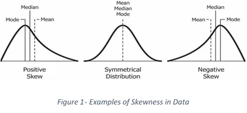
3. Skewness
The shape of a distribution matters. Some distributions are symmetric, like the familiar bell curve, but real data are often lopsided, leaning to the left or right. Skewness measures how asymmetric a distribution is. Because the mean, median and mode all describe the centre of a dataset, the way they relate to one another reveals the skew. In a right-skewed (positively skewed) distribution the mean is typically greater than the median; in a left-skewed (negatively skewed) distribution the mean is typically less than the median.
When to use it: to check distribution shape before choosing an inferential test, since many tests assume an approximately normal distribution. Judging skew from a graph alone is subjective, so it is best calculated numerically — for example, with Pearson’s coefficient of skewness.
Part 2: Inferential Statistics
Inferential statistics let you use data from a sample to draw conclusions about a larger population. This is where you test whether the patterns you described are likely to be real rather than a product of chance. The four techniques below — hypothesis testing, correlation, regression and ANOVA — cover the vast majority of beginner dissertation analyses.
4. Hypothesis Testing
Hypothesis testing assesses whether a specific claim about a population is supported by your data. You state a null hypothesis (usually “no effect” or “no difference”) and an alternative hypothesis, then use a test such as the t-test or chi-square test to decide which is more credible. The result is judged statistically significant if the observed effect would be very unlikely to occur by random chance alone, conventionally when the p-value is below 0.05.
When to use it: to compare groups or test a claim — for example, whether a new teaching method produces higher scores than the standard one. Tests can be run easily in SPSS or Minitab.
5. Correlation
Correlation analysis studies the strength and direction of a relationship between two continuous variables. It is summarised by a correlation coefficient (commonly Pearson’s r) ranging from -1 to +1: a value near +1 indicates a strong positive relationship, near -1 a strong negative relationship, and near 0 little or no linear relationship. Importantly, correlation does not imply causation — two variables can move together without one causing the other.
When to use it: to see whether two numeric variables move together, such as hours studied and exam marks. For ordinal data, Spearman’s rank correlation is the appropriate alternative.
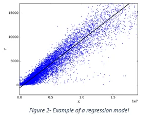
6. Regression
Regression goes a step beyond correlation by modelling how one variable predicts or explains another. The simplest form, simple linear regression, fits the “best” straight line between an independent (explanatory) variable and a dependent variable, usually shown on a scatterplot. The fitted line takes the form y = a + bx, where b is the slope (the predicted change in y for each one-unit increase in x) and a is the intercept.
When to use it: when you want to predict or quantify the effect of one variable on another — for example, predicting sales from advertising spend. Multiple regression extends this to several predictors at once.
7. ANOVA (Analysis of Variance)
A t-test compares the means of two groups, but when you have three or more groups, running multiple t-tests inflates the chance of a false positive. Analysis of variance (ANOVA) solves this by testing, in a single test, whether the means of three or more groups differ significantly. A significant result tells you that at least one group mean differs from the others; follow-up (post-hoc) tests then identify which.
When to use it: to compare averages across three or more groups — for example, comparing mean exam scores across four different schools. One-way ANOVA handles a single grouping factor; two-way ANOVA handles two.
How to Choose the Right Statistical Test
Choosing a test comes down to three questions: what type of data do you have, how many groups or variables are involved, and what are you trying to find out (describe, compare or predict)? The flowchart below summarises the decision for the most common beginner scenarios. For a fuller treatment, see our guide on which statistical test you should use.
Choosing a statistical test
- Describe one variable? Use the mean and standard deviation (plus skewness to check shape).
- Relationship between two numeric variables? Use correlation, then regression if you want to predict.
- Compare two group means? Use a t-test.
- Compare three or more group means? Use ANOVA.
- Test a claim about a population? Use hypothesis testing with an appropriate significance level.
Struggling with your dissertation statistics?
ResearchProspect to the rescue!
Our expert statisticians can run, interpret and write up your analysis correctly — explore our statistical analysis service to get matched with a specialist.

How ResearchProspect Can Help
Whether you are an undergraduate, Master’s or PhD student, our expert statisticians can help with every part of your data analysis, from choosing the right test to interpreting the output and writing up the findings chapter. However urgent or complex your needs, our large team of statistical consultants means we can assign a suitable expert to your order. You can read genuine client feedback on our reviews page before you decide.


