


A Type I error is a false positive: you reject a null hypothesis that is actually true (rejecting H₀ when H₀ is correct). A Type II error is a false negative: you fail to reject a null hypothesis that is actually false (keeping H₀ when the alternative is true). The probability of a Type I error is the significance level, α; the probability of a Type II error is β. Every hypothesis test risks exactly these two mistakes, and the two examples below show why getting them right matters.
When testing a hypothesis, you first state a null hypothesis. The null hypothesis (denoted H₀) proposes that there is no real effect, difference or relationship between the variables in the population — any pattern in your sample is just chance. Researchers usually hope to reject the null in favour of an alternative hypothesis (denoted H₁ or Hₐ), which states that a genuine effect does exist.
Because a test only ever sees a sample rather than the whole population, its conclusion is a probabilistic bet — and that bet can be wrong in two distinct ways. Consider a simple research question:
Question: Is the COVID-19 vaccine safe for people with heart conditions?
Null Hypothesis (H₀): The vaccine has no effect on safety outcomes for people with heart conditions.
Alternative Hypothesis (H₁): The vaccine changes safety outcomes for people with heart conditions.
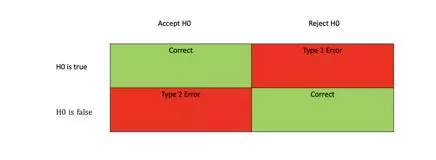
Whatever the test decides, reality is fixed but unknown. This gives four possible outcomes — two correct, two mistaken — which are best shown as a 2×2 decision table comparing the truth against your decision.
Correct ✓
False positive
False negative
Correct ✓
| Decision: Fail to reject H₀ | Decision: Reject H₀ | |
|---|---|---|
| Truth: H₀ is true (no real effect) | Correct decision (true negative), probability 1−α |
Type I error (false positive), probability α |
| Truth: H₀ is false (real effect exists) | Type II error (false negative), probability β |
Correct decision (true positive), probability 1−β = power |
The two error cells sit on the diagonal: a Type I error lives in the top-right cell (you acted when you should not have), and a Type II error lives in the bottom-left cell (you failed to act when you should have). The two correct cells make up the rest. Keep this table in mind for everything that follows.
“In a test of a statistical hypothesis, a Type I error is the error of rejecting the null hypothesis when it is true, and a Type II error is the error of failing to reject the null hypothesis when it is false.” — NIST/SEMATECH e-Handbook of Statistical Methods (U.S. National Institute of Standards and Technology)
Understanding the Type I Error (False Positive, α)
A Type I error occurs when you reject the null hypothesis even though it is actually true. In plain terms, you conclude there is a real effect, difference or relationship when in fact there is none — a false positive. This is why a Type I error is also called a false alarm.
The probability of making a Type I error is set in advance by you and is called the significance level, written as the Greek letter alpha (α). The most common choice is α = 0.05, meaning you accept a 5% risk of a false positive. In any single test, the p-value is compared against α: if p ≤ α, you reject H₀. So choosing α = 0.05 means that, if the null were true, you would wrongly reject it about 5 times in 100. Lowering α to 0.01 cuts the false-positive risk to 1%, but — as we will see — makes a Type II error more likely. The relationship between α and the evidence threshold is explored further in our guide to statistical significance.
- What it means: rejecting a true null — “crying wolf”.
- Symbol: α (alpha), the significance level.
- Controlled by: the researcher, before collecting data.
- Reduce it by: choosing a smaller α (e.g. 0.01 instead of 0.05), or correcting for multiple comparisons.
Worked Example — Type I Error
Real-world Type I errors are usually subtler than this, but the structure is always the same: the null is true, yet the test says “reject”.
Is the statistics assignment pressure too much to handle?
How about we handle it for you?
Put in your order right now to save yourself time, money and last-minute stress.
Understanding the Type II Error (False Negative, β)
A Type II error occurs when you fail to reject the null hypothesis even though it is actually false. In other words, a real effect or difference genuinely exists in the population, but your test does not detect it — so you conclude “no effect” when there really is one. This is a false negative, sometimes called a miss.
The probability of a Type II error is denoted by the Greek letter beta (β). Beta is directly tied to the power of a statistical test:
- What it means: failing to reject a false null — missing a real effect.
- Symbol: β (beta); power = 1 − β.
- Driven by: sample size, true effect size, data variability and α.
- Reduce it by: increasing power — see below.
How to Reduce a Type II Error
Because β = 1 − power, the way to reduce a Type II error is to increase the power of your test. There are several practical levers:
- Increase the sample size. This is the most reliable lever. A larger sample gives a more precise estimate and a smaller standard error, making genuine effects easier to detect. In the coin example below, using n = 200 instead of n = 100 raises the power.
- Increase the significance level α. Using α = 0.05 instead of α = 0.01 lowers the evidence bar for rejecting H₀, which raises power and reduces β — but it deliberately increases the Type I error rate. It is a trade-off, not a free lunch.
- Detect a larger true effect. Bigger real effects are easier to detect, so power is higher when the true effect is far from the null value.
- Reduce variability. Tighter measurement and better study design shrink the standard error and lift power.
Note that increasing the sample size raises power without increasing the Type I error rate, which is why it is the preferred fix. For the full picture, see our dedicated guide to statistical power.
Worked Example — Type II Error
A common point of confusion: a small β means a low chance of a Type II error, not a high one. If β = 0.03, the probability of a Type II error is just 3%, and the test’s power is a strong 97%. Beta and power always add to 1.
How Type I, Type II, Power and Significance Fit Together
The four quantities are locked into a single trade-off. Significance (α) controls false positives; β controls false negatives; power (1 − β) is the test’s ability to find a true effect. The table below summarises them.
| Concept | Symbol | What it measures | Plain meaning |
|---|---|---|---|
| Significance level | α | P(reject H₀ | H₀ true) | Type I error rate (false positive) |
| Confidence | 1 − α | P(fail to reject H₀ | H₀ true) | Correctly keeping a true null |
| Type II error rate | β | P(fail to reject H₀ | H₀ false) | False negative (a miss) |
| Power | 1 − β | P(reject H₀ | H₀ false) | Correctly detecting a real effect |
The key tension: lowering α reduces Type I errors but, all else equal, raises β (more Type II errors). You cannot drive both to zero at once with a fixed sample. The escape route is to increase the sample size, which lifts power and lowers β without inflating α. Choosing α is therefore a judgement about which error is more costly in your specific context — the subject of the next section.
Which is Worse — Type I or Type II Error?
The honest answer is: it depends entirely on the consequences of each mistake in the situation at hand. Neither error is universally worse; you weigh the real-world cost of a false positive against the cost of a false negative.
Medical screening example. Imagine a screening test for diabetes, where H₀ is “the patient does not have diabetes”.
- A Type I error (false positive) tells a healthy patient they may have diabetes. This causes worry and triggers further tests, but those follow-up checks usually reveal the truth, so the harm is often limited.
- A Type II error (false negative) tells a patient with diabetes that they are healthy. They may skip treatment and the illness can progress untreated — a far more dangerous outcome.
Here, the Type II error (the false negative) is the more serious one, so the test is designed to keep β low even at the cost of more false positives.
Courtroom example. In a criminal trial under “innocent until proven guilty”, H₀ is “the defendant is innocent”.
- A Type I error (false positive) means rejecting innocence when the defendant truly is innocent — convicting an innocent person.
- A Type II error (false negative) means failing to reject innocence when the defendant is in fact guilty — letting a guilty person go free.
Most legal systems treat convicting the innocent (the Type I error) as the worse outcome — captured in Blackstone’s principle that it is better that ten guilty persons escape than that one innocent suffer — so the burden of proof is set deliberately high. The contrast with the medical case shows the same statistics can favour opposite priorities depending on what is at stake.
Worried about Type I and Type II errors in your analysis?
ResearchProspect to the rescue!
Our statisticians will design your test, set the right α and power, and interpret the results — explore our statistical analysis service.


