


What is a Normal Distribution?
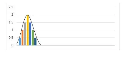
A normal distribution is a continuous probability distribution that is perfectly symmetric about its mean, where data points cluster most densely around the centre and become progressively rarer towards the tails. When plotted, it forms the familiar bell-shaped curve — the answer to the common multiple-choice question is that a normal distribution is a symmetric, bell-shaped curve, not skewed, uniform or flat. It is also called the Gaussian distribution after Carl Friedrich Gauss.
In a normal distribution, the mean, median and mode are all equal and sit at the centre of the curve. Exactly 50% of the data lies to the left of the mean and 50% to the right. Many natural and social phenomena — heights, blood pressure, exam scores and measurement errors — approximate this shape, which is why it is the single most important distribution in statistics.
“The normal distribution is a probability function that describes how the values of a variable are distributed. It is a symmetric distribution where most of the observations cluster around the central peak and the probabilities for values further away from the mean taper off equally in both directions.” — National Library of Medicine (NIH), StatPearls
Data, of course, can be distributed in several ways. It can lean to the left (negatively skewed), lean to the right (positively skewed), or be spread symmetrically with no skew. Only the symmetric, skew-free case produces a true normal distribution.
- Left-skewed (negative skew): a longer tail on the left; the mean is pulled below the median.
- Right-skewed (positive skew): a longer tail on the right; the mean is pulled above the median.
- Symmetric (no skew): the two halves mirror each other — this is the normal distribution.
Note: Skewness in statistics is the asymmetry or distortion of a distribution away from the perfect bell curve. A normal distribution has a skewness of zero. For a fuller picture of how spread and centre interact, see our guides on measures of variability and descriptive statistics.
History of the Normal Distribution
The roots of the normal distribution lie in the study of measurement error. As early as the 17th century, astronomers including Galileo observed that the errors in their measurements followed a consistent pattern: small errors occurred far more often than large ones, and errors of equal size were equally likely in either direction.
The mathematics was formalised over the following centuries. Abraham de Moivre derived the curve as an approximation to the binomial distribution in 1733, and in the early 19th century Carl Friedrich Gauss and Pierre-Simon Laplace developed it into the theory of errors we use today — which is why the distribution is named after Gauss. The term “normal” was popularised later by Karl Pearson around the turn of the 20th century.
The alternative name probability density distribution captures the intuition well: because a small error is more probable than a large one, the probability is densest around the mean of the measurements and thins out towards the tails.
Properties of a Normal Distribution
Every normal distribution shares the same core properties, regardless of its mean or standard deviation:
- The mean, median and mode are all equal and lie at the centre.
- The curve is perfectly symmetric about the mean.
- Exactly half of the values fall below the mean and half above it.
- The total area under the curve equals 1 (i.e. 100% of the probability).
- The curve is asymptotic — the tails approach the x-axis but never quite touch it, so the distribution extends infinitely in both directions.
- The distribution is fully described by just two parameters: the mean and the standard deviation.
Parameters of the Normal Distribution
A normal distribution is defined by exactly two parameters: the mean (μ) and the standard deviation (σ). Together these determine where the curve sits and how wide it is. Changing them shifts and stretches the bell, but never changes its essential symmetric, bell-shaped form.
The mean is a location parameter — it fixes the central point and therefore the position of the peak along the x-axis. The standard deviation is a scale parameter — it controls the spread, or width, of the curve. A large standard deviation produces a wide, flat curve; a small standard deviation produces a narrow, tall one.
Mean
The mean is a measure of central tendency, best suited to variables measured on interval or ratio scales. In a normal distribution graph the mean defines the peak — the point around which all other data points are arranged. Increasing or decreasing the mean slides the entire curve right or left along the x-axis without changing its shape.
Standard Deviation
The standard deviation measures how far, on average, data points lie from the mean. On the graph it controls the width of the curve. A small standard deviation gives a narrow, steep bell because values are tightly packed around the mean; a large standard deviation gives a wide, flatter bell because values are more spread out. As the standard deviation changes, the curve tightens or widens along the x-axis while the area beneath it stays fixed at 1.
| Parameter | Symbol | Role | Effect on the curve |
|---|---|---|---|
| Mean | μ | Location parameter | Moves the peak left or right along the x-axis |
| Standard deviation | σ | Scale parameter | Widens (large σ) or narrows (small σ) the curve |
Why the Normal Distribution Matters
The normal distribution appears throughout the natural and social sciences. It closely models variables such as human height, birth weight, blood pressure, exam marks, reaction times and measurement errors. Its real significance, however, comes from the central limit theorem, which explains why so many statistical methods rely on it.
The Central Limit Theorem
The central limit theorem (CLT) states that if you take sufficiently large random samples from any population with a finite variance, the distribution of the sample means will be approximately normal — regardless of the shape of the original population. As the sample size grows, that approximation becomes more accurate.
This is profoundly useful: it means we can apply normal-distribution-based methods (confidence intervals, z-tests and many others) to sample data even when the underlying population is not itself normal. The CLT underpins much of inferential statistics and explains why the normal curve turns up so often in practice. To see how it informs the leap from sample to population, read our guides on population vs sample and the standard error.
The Normal Distribution Formula
The probability density function of a normal distribution is:
f(x) = (1 / (σ√(2π))) · e−(x − μ)2 / (2σ2)
where:
- f(x) = the probability density at value x
- x = the value of the variable
- μ = the mean
- σ = the standard deviation
- σ2 = the variance
- π ≈ 3.14159
- e ≈ 2.71828 (Euler’s number)
The 68-95-99.7 Empirical Rule
The empirical rule (also called the 68-95-99.7 rule or the three-sigma rule) describes how data is spread in any normal distribution. It tells you what proportion of values lie within a given number of standard deviations of the mean:
- About 68% of values lie within 1 standard deviation of the mean (μ ± 1σ).
- About 95% of values lie within 2 standard deviations of the mean (μ ± 2σ).
- About 99.7% of values lie within 3 standard deviations of the mean (μ ± 3σ).
| Range | Interval | Approx. % of data |
|---|---|---|
| ± 1 standard deviation | μ − σ to μ + σ | 68% |
| ± 2 standard deviations | μ − 2σ to μ + 2σ | 95% |
| ± 3 standard deviations | μ − 3σ to μ + 3σ | 99.7% |
• 68% of people score within 1σ of the mean → between 100 − 15 = 85 and 100 + 15 = 115.
• 95% score within 2σ → between 100 − 30 = 70 and 100 + 30 = 130.
• 99.7% score within 3σ → between 100 − 45 = 55 and 100 + 45 = 145.
Because the curve is symmetric, the 68% within 85–115 splits evenly: 34% lie between 85 and 100, and 34% between 100 and 115. Only about 0.3% of people score below 55 or above 145 combined — the rare tails of the distribution.
To go further and calculate the probability for any value (not just whole standard deviations), you convert your data to z-scores and use the standard normal distribution, which has a mean of 0 and a standard deviation of 1.
Struggling to analyse your data?
ResearchProspect to the rescue!
Our experts can run, interpret and write up your distributions, tests and models — explore our statistical analysis service.

Key Takeaways
- A normal distribution is a symmetric, bell-shaped probability distribution — not skewed, uniform or flat.
- It is symmetric about its centre, where the mean = median = mode.
- Exactly half the values lie below the mean and half above it; the total area under the curve is 1.
- It is fully defined by two parameters: the mean (location) and the standard deviation (spread).
- The empirical rule says roughly 68%, 95% and 99.7% of data fall within 1, 2 and 3 standard deviations of the mean.
- The central limit theorem explains why sample means tend towards normality, making the distribution central to inferential statistics.


