Disclaimer: This is not a sample of our professional work. The paper has been produced by a student. You can view samples of our work here. Opinions, suggestions, recommendations and results in this piece are those of the author and should not be taken as our company views.
Type of Academic Paper – Report
Academic Subject – Chemical Engineering
Word Count – 2707 words
The instrumentation and the control laboratory experimentation provided a good outline for the dynamic behaviour of equipment and the feedback controller.
The experiment was conducted on a surge tank control system equipped with a tank and installed level sensor, a pump, a control valve, and a digital flow meter in the outlet stream.
First, the level sensor was calibrated using an Auto mode by progressively changing the setpoints (level %) and recording the measured signals (volts). The extent of hysteresis was also assessed using increasing and then decreasing liquid levels. The results showed that the sensor does not have a high hysteresis error, and it responds well with a change in the liquid level.
The control Valve was then calibrated using the Manual mode and changing the inlet variable (signal from the controller in %) progressively and recording the output variable (flow rate through the valve). The extent of hysteresis was also assessed. Plots of the valve characteristics showed that the valve could only work in a small range when setting on Manual mode, and the valve had a huge hysteresis error. It needed to be reinstalled and replaced to get the desired results. The practical observation also determined that the control valve was Fail open (F.O.) as it opens when no signal is obtained from the level sensor.
The feedback control loop, the importance of automatic tuning, and each term’s effect in a three-term controller on the control performance was analysed. The performance of default control parameters by changing the three controller parameters was observed. It was concluded that each parameter’s effect on the system depends on various parameters and the system’s characteristics. Tuning set parameters gives stabilised P.I.D. parameters.
Digital instrumentation and control have proven to be very useful in many industries and are beneficial in a wide range of applications. This usefulness is evidence of the trend of investment in digital instrumentation and control applications in the process industry over the last 20 years (Astrom and Hagglund, 2005). Investment in automatic control systems is an important element in achieving optimal plant performance.
Instrumentation controls are the apparatuses used to measure physical variables such as level, density, pressure, flow current, voltage, and chemical properties of a substance or a product (Alberto, 2005). The most important and basic function of instrumentation control is to measure and calculate the various devices’ response. The control systems ensure that the system’s mechanism is running smoothly and the entire variables are controlled as per the process requirements.
The laboratory experiment’s main objective was to introduce ourselves to the pilot-scale equipment’s dynamic behaviour and the operation of the feedback controller. Understanding the feedback loop’s role and operation consisting of sensor, actuator, and controller was the principal aim.
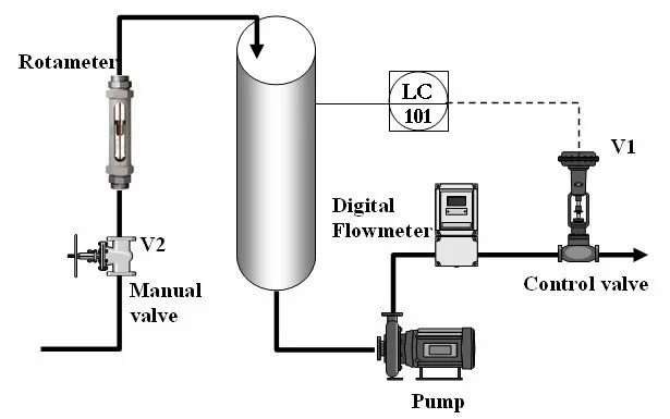
Figure 1. Flow diagram of the level control system
The plant consisted of a liquid surge tank with a control valve and a pump in the outlet stream. The flow into the tank was independent of the liquid in the tank and could be set by a traditional flow meter.
The outlet flow was measured by a digital flow meter connected just before the control valve in the outlet stream. The tank’s flow was also independent of the tank’s liquid level (to a certain approximation), resulting in the tank acting as an integrator of the difference between the flow rates. Hence control action was needed to stabilise the liquid level (restricting it from overflowing) by making one of the flow rates dependent on the liquid level.
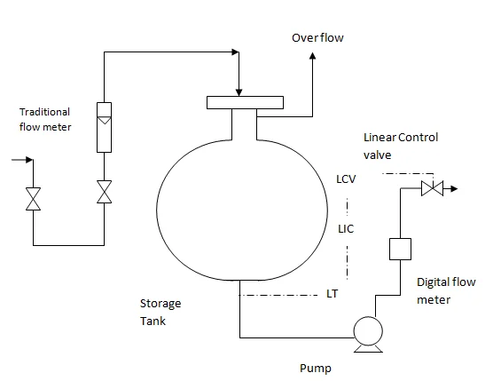
Figure 2. Process and Instrumentation Diagram of the System
The objectives of the laboratory were as follows:
(1) Calibrate the level sensor in the feedback loop.
(2) Calibrate the control valve and study the installed characteristics of a valve.
(3) Study the effect of hysteresis in the control valve and sensor.
(4) Understand the dynamic behaviour of the system.
(5) Evaluate manual control.
(6) Evaluate the tuning of a P.I.D. control via manual and automatic tuning.
(7) Evaluate the effect of positive or negative feedback on the closed-loop system
The level sensor is an electronic linear device that sends a usually electric signal, depending on the level in the storage tank (Visioli, 2006). The sensor’s calibration was completed by correlating signal value (volts) to the tank’s real volume. First, the range of operation of the sensor’s input variable (the liquid level in the tank) and the output signal sent to the controller was determined by setting the controller to auto mode and then changing the set point on the computer to a maximum and then minimum values (10 and 90%). The values were noted after stabilising the system to reduce errors.
Then starting from the minimum value, the setpoints were changed progressively covering the complete range, and the values of the level (in %) and the output valued from the sensor (in volts) were recorded.
The extent of hysteresis was calibrated through increasing liquid levels and then reversing the process using falling liquid levels.
The control valve is a device that affects fluid or gas flow and pressure through a closed system (Jelali, 2006). It changes the flow of fluid by altering its resistance by changing the external signals. A control valve consists of two main components; (1) the valve actuator which accepts external signals and changes the stem position and flow rate. (2) Valve action which contains a movable plug attached to the valve system. By partially blocking the valve orifice with the valve plug, variable flow resistance is obtained. They are either Fail Open, producing maximum flow at a minimum signal or Fail Close, producing minimum flow at the minimum.
It contains an orifice and movable plug, which provides resistance to the flow through the valve. The fluid flow variation concerning the valve plug movement can be different for various valves, and their characteristics can define it.
The controller was set on manual mode, and the manual control input in the interface was set so that the valve was fully open. Then the inlet flows into the tank were increased by adjusting the hand valve below the flow meter. A steady-state maximum level is achieved in the tank (as the water was overflowing, keeping the tank at maximum level). This step was completed to ensure that any effect of change in the tank’s level on the flow rate through the control valve is eliminated.
The range of the output variable (flow rate) was then determined by setting the input variable (signal from the controller) to a maximum and minimum value 0 and 100%. The values of the corresponding flow rates were determined.
Then the input variable was set at several points covering the range, and the flow rate values were determined to form the electronic flow rate installed in the output line. The extent of hysteresis was also analysed by calibrating the process by increasing the input signal and then decreasing the sign.
The controller was set on ‘auto mode’, and the liquid was defined to a set point. After letting the system stabilise, the controller was set to manual mode, and the setpoint was changed. With the action of buttons in the process diagram pane, the new level was maintained to a certain approximation, and it was repeated certain times, and the observation was analysed.
The Three-term controllers Proportional Integral derivatives (P.I.D.) are mostly used in process industries (Skogestad, 2006). It calculates the difference between the measured signal and the set value and consequently changes the valve position to reduce the error. The three parameters are proportional gain (Kc), integral time (T1), and derivative time (T.D.).
The controller was set on auto mode, and after letting it get stabilised to the desired setpoint, the three components were changed for different set points, and their performances were tested. Over shoots, time to reach the setpoint, steady-state errors, and the control action’s speed together with the variation in the water level were also observed and analysed.
The three P.I.D. parameters were modified one by one by one in the later stage. First, the P only was tested by setting Ti and Td equal to zero. Then Kc was set as constant, Td was set to zero Ti was varied. Finally, Kc and Ti were set as constant and Td was varied to obtain the results.
After setting control mode on auto and letting the system stabilise at the desired setpoint, the Automatic Tuning Wizard tool was started, and the tuning procedure was completed. At the end of the procedure, the new parameters were automatically saved into the controller panel’s P.I.D. parameters tag. The new controller parameters were recorded, and the control performance was tested again. The PPI and P.I.D. control structures were tuned with fast, slow, and normal actions.
Orders completed by our expert writers are

Various sensor calibration methods were adopted to produce sensor behaviour results: increasing tank levels and decreasing tank levels used in the experiments. Hysteresis factor is an effective means for the quantification of sensor behaviour. Signal levels were determined from system processing and analysed to obtain the system sensitivity.
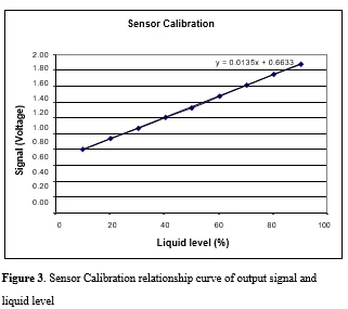
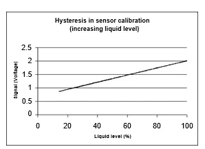
Figure 4. Hysteresis in sensor calibration for increasing liquid level in the storage tank
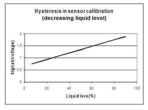
Figure 5. Hysteresis in sensor calibration for decreasing liquid level in the storage tank
The results in Figures 3 to 5 show that the level sensor starts responding from the value of 0.633 volts and reaches to a maximum amount of 2 volts approximately. The level sensor is also more sensitive while increasing the liquid level (hysteresis). The sensor (or the gain) is 0.0135 volts per 1% increase in the fluid level.
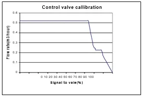
Figure 6. Hysteresis in sensor calibration for decreasing liquid level in the storage tank
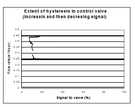
Figure 7. Hysteresis output in control valve for varying liquid level in the storage tank
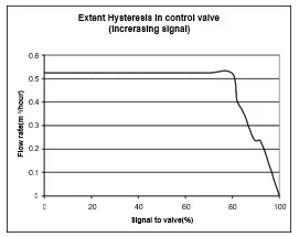
Figure 8. Hysteresis output in control valve for increasing signal to control Valve
The recorded values and the plots show that the control valve malfunctions in a particular range. When set on manual mode, it only operates in a very narrow range, between 80 to 100%. The control valve also behaves differently when working with increasing and decreasing the signal strength, concluding that the system has a high hysteresis error.
Different values were obtained for the flow rate through the control valve at the same input signal (as the procedure was repeated multiple times). The best values were used to calculate the plots shown above.

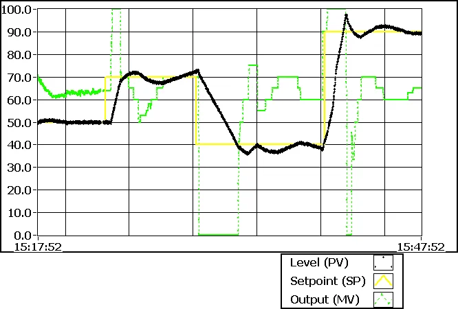
Figure 9. The change in Tank level to change in the Setpoint with manual control
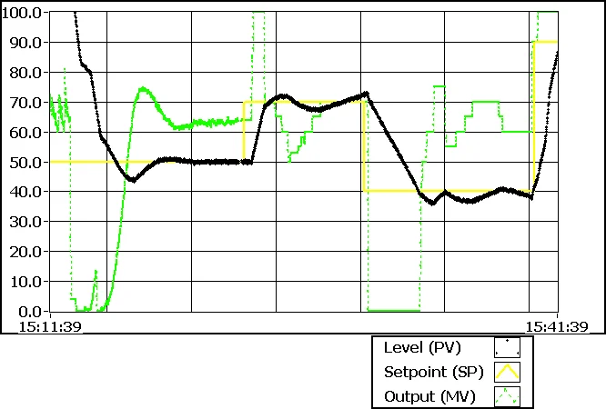
Figure 10. The change in Tank level concerning the difference in the Setpoint with manual control
To get the tank’s level close to that set value, a larger% change to the control valve had to be made as the level sensor was not very sensitive.
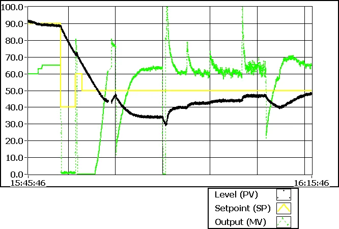
Figure 11. Tank level to change in the Setpoint
When Ti and Td are kept are 0 value, and changing Kc’s values, the volume in the tank never touches the setpoint value. Increasing Kc reduces error, but it dramatically increases the valve body vibration, which might cause damage to Valve.

Figure 12. Volume variation with changing control inputs
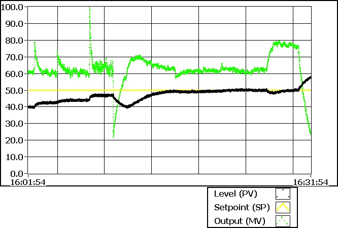
Figure 13. Volume variation with changing control inputs
Fixing Kc and varying but keeping Td = 0 shows that Ti’s increase does not considerably change the volume. It shows a steady-state error with low %, and it also reaches close to the Setpoint at a reasonable rate. By changing Ti, the vibration in the Valve is not affected.
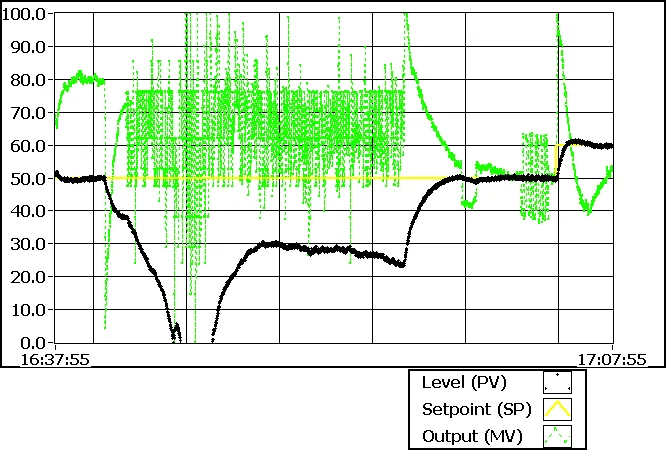
Figure 14. Volume response with changing control inputs
By fixing Kc and Ti but varying Td increases the error. Reducing the Td value decreases the mistake and the vibration in the Valve.
Tuning the set parameters increases the valve body’s vibration without any change in % error and gives stabilised P.I.D. or P.I parameters.
When the valve is fully open, Valve’s maximum flow rate is 0.532 m3/hour. If the inlet flow rate exceeds this value, the system will never stabilise because the tank will act as an integral of the flow rate difference.
Changing the sign of the controller gain Kc completely alters the system, as shown below in the diagram
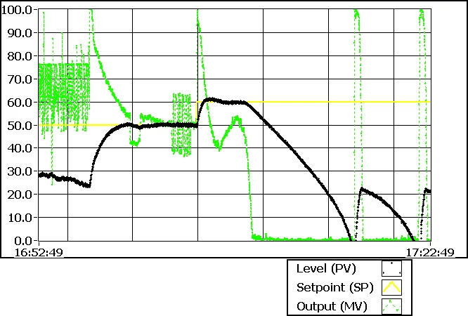
Figure 15. System response with a negative input control
For the valve actuator;
x = a.u +b, where a and b are constants, x is the stem position, and you are input signal.
Digital instrumentation and control of the fluid level system can be utilized through feedback control. The effluent flow and level in the tank can be controlled through adjustment in the control variables.
A schematic Proportional, Integral, and derivative controls were applied to the level tank fluid transfer system. The results showed that the system performance could be optimised to apply optimum control parameters and values. The system’s experimental analyses showed that the level sensor starts responding from the output value of 0.633 volts and reaches to a maximum value of 2 volts during operations. The sensor’s sensitivity was observed as 0.0135 volts for every one per cent increase in the liquid level under steady-state conditions. The control valve operation range was determined to be between 80 to 100% when operating under manual mode. Automatic fine-tuning of the control parameters resulted in increased vibration of the valve body. However, stabilised P.I.D. or P.I parameters can be obtained through manual and automatic tuning of the system parameter.
Alberto, L., 2005. Auto tuning process controller with improved load disturbance rejection. J. Process Control, 15, 223−234
Astrom, K. J and Hagglund, T., 2005. Advanced P.I.D. Control; International, Society of Automation: Research Triangle Park, NC.
Hagglund, T., 2005. Industrial implementation of on-line performance monitoring tools. Control Eng. Pract.
Jain, M., and Lakshminarayanan, S., 2005. A filter-based approach for performance assessment and enhancement of SISO control systems.Ind. Eng. Chem. Res.
Jalali, M., 2006. An overview of control performance assessment technology and industrial applications. Control Eng. Pract, 14, 441−466
Ko, B. S., and Edgar, T. F., 2004. P.I.D. Control performance assessment: The single-loop case. AIChE J.
Michael, W. F., Julien, R. H., and Brian, R. C., 2005. A comparison of P.I.D. Controller tuning methods. Can. J. Chem. Eng, 83, 712−722.
Peter, K., and Alexander, H., 2005. Detection of sluggish control loops: experiences and improvements. Control Eng. Pract. 1029−1025.
Skogestad, S., 2006. Tuning for smooth P.I.D. Control with acceptable disturbance rejection. Ind. Eng. Chem. Res, 45, 7817−7822
Visioli, A., 2006. Method for proportional-integral controller tuning assessment. Ind. Eng. Chem. Res, 45, 2741−2747
If you are the original writer of this Report and no longer wish to have it published on the www.ResearchProspect.com then please:
To write an undergraduate academic report:

All work is written by human writers. 100% AI free, guaranteed.

100% money back guarantee if you find plagiarism in our work.
COMPANY DETAILS


